DVH Metrics¶

Dose-volume histogram metrics summarize the dose received by a structure. A cumulative DVH reports, for every dose level \(D\), the percentage of structure voxels receiving at least that dose:

\[ \mathrm{DVH}(D) =100\,\frac{\left|\left\{v\in V_{\mathrm{structure}}:d(v)\geq D\right\}\right|} {\left|V_{\mathrm{structure}}\right|}. \]

Try DVH analysis

Complete DVH API classification¶

Every public function in dosemetrics.metrics.dvh is listed below.

Reference-free computations¶

Function	Result
`compute_dvh`	Dose bins and cumulative volume percentages for one dose and structure
`compute_volume_at_dose`	\(V_x\): percentage receiving at least a dose threshold
`compute_dose_at_volume`	\(D_x\): dose received by at least a percentage of the volume
`compute_dose_at_volume_cc`	Dose to the hottest requested absolute volume
`compute_equivalent_uniform_dose`	Equivalent uniform dose for a tissue-response parameter
`compute_dose_statistics`	Mean, maximum, minimum, median, standard deviation, and selected \(D_x\) values
`compute_mean_dose`	Mean structure dose
`compute_max_dose`	Maximum structure dose
`compute_min_dose`	Minimum structure dose
`compute_median_dose`	Median structure dose
`compute_dvh_auc`	Area under one cumulative DVH
`compute_dose_percentile`	Dose percentile using the clinical \(D_x\) convention
`compute_dvh_confidence_interval`	Mean DVH and percentile interval across multiple doses
`compute_dvh_bandwidth`	Pointwise maximum-minus-minimum DVH band across multiple doses
`create_dvh_table`	Long-form DVH table for a `StructureSet`
`extract_dvh_metrics`	Selected \(D_x\) and \(V_x\) values in one dictionary

Reference-based comparisons¶

Function	Result
`dvh.compare_dvh_score` / direct `compare_dvh_score` export	Complete OpenKBP DVH Score
`compare_dvh_wasserstein`	Wasserstein distance between structure dose samples
`compare_dvh_area`	Integrated L1 or L2 separation between cumulative DVHs
`compare_dvh_chi_square`	Chi-square statistic and p-value for differential DVHs
`compare_dvh_ks`	Two-sample Kolmogorov-Smirnov statistic and p-value
`compare_dvh_similarity`	Dice, Jaccard, correlation, or cosine similarity between DVHs
`dvh.compare_oar_dvh_auc` / direct `compare_oar_dvh_auc` export	Absolute difference between two OAR DVH AUCs
`dvh.compare_mean_oar_dvh_auc` / direct `compare_mean_oar_dvh_auc` export	Mean OAR DVH AUC distance over a collection

Construct a DVH¶

from dosemetrics.metrics import dvh

dose_bins, volume_percent = dvh.compute_dvh(
    dose, ptv, step_size=0.1, verbose=True
)

dose_bins is measured in Gy and volume_percent ranges from 0 to 100. verbose=True prints a one-line summary; it is silent by default.

Dose-at-volume and volume-at-dose¶

The dose received by at least \(x\%\) of the structure is \(D_x\):

\[ D_x=\inf\left\{D:\mathrm{DVH}(D)\leq x\right\}. \]

d95 = dvh.compute_dose_at_volume(dose, ptv, volume_percent=95)
d2 = dvh.compute_dose_at_volume(dose, ptv, volume_percent=2)
d01cc = dvh.compute_dose_at_volume_cc(dose, spinal_cord, volume_cc=0.1)

The percentage receiving at least \(x\) Gy is \(V_x\):

v20 = dvh.compute_volume_at_dose(dose, lung_left, dose_threshold=20.0)

Dose statistics¶

stats = dvh.compute_dose_statistics(dose, ptv, verbose=True)

The scalar helpers compute_mean_dose, compute_max_dose, compute_min_dose, and compute_median_dose return the corresponding entry without building the full dictionary.

For several structures at once, use the display- and export-ready helper:

from dosemetrics.utils import dose_statistics_table

table = dose_statistics_table(dose, structures, ["PTV", "Brainstem"])

Equivalent uniform dose¶

For \(N\) structure voxels and tissue-response parameter \(a\),

\[ \mathrm{EUD}=\left(\frac{1}{N}\sum_{i=1}^{N}d_i^a\right)^{1/a}. \]

eud_target = dvh.compute_equivalent_uniform_dose(dose, ptv, a_parameter=-10.0)
eud_oar = dvh.compute_equivalent_uniform_dose(dose, spinal_cord, a_parameter=8.0)

Single-plan DVH AUC¶

compute_dvh_auc integrates a single cumulative DVH. With normalize=True, it divides by the maximum possible area over the selected dose range and returns a value from 0 to 1. With normalize=False, it returns the trapezoidal integral in Gy·%.

\[ \mathrm{AUC}=\int_{D_{\min}}^{D_{\max}}V(D)\,\mathrm{d}D. \]

normalized_auc = dvh.compute_dvh_auc(dose, brainstem, normalize=True)
auc_gy_percent = dvh.compute_dvh_auc(dose, brainstem, normalize=False)

PTV mean-dose distance¶

Reference-based · compare_ptv_dose · Gy · lower is better.

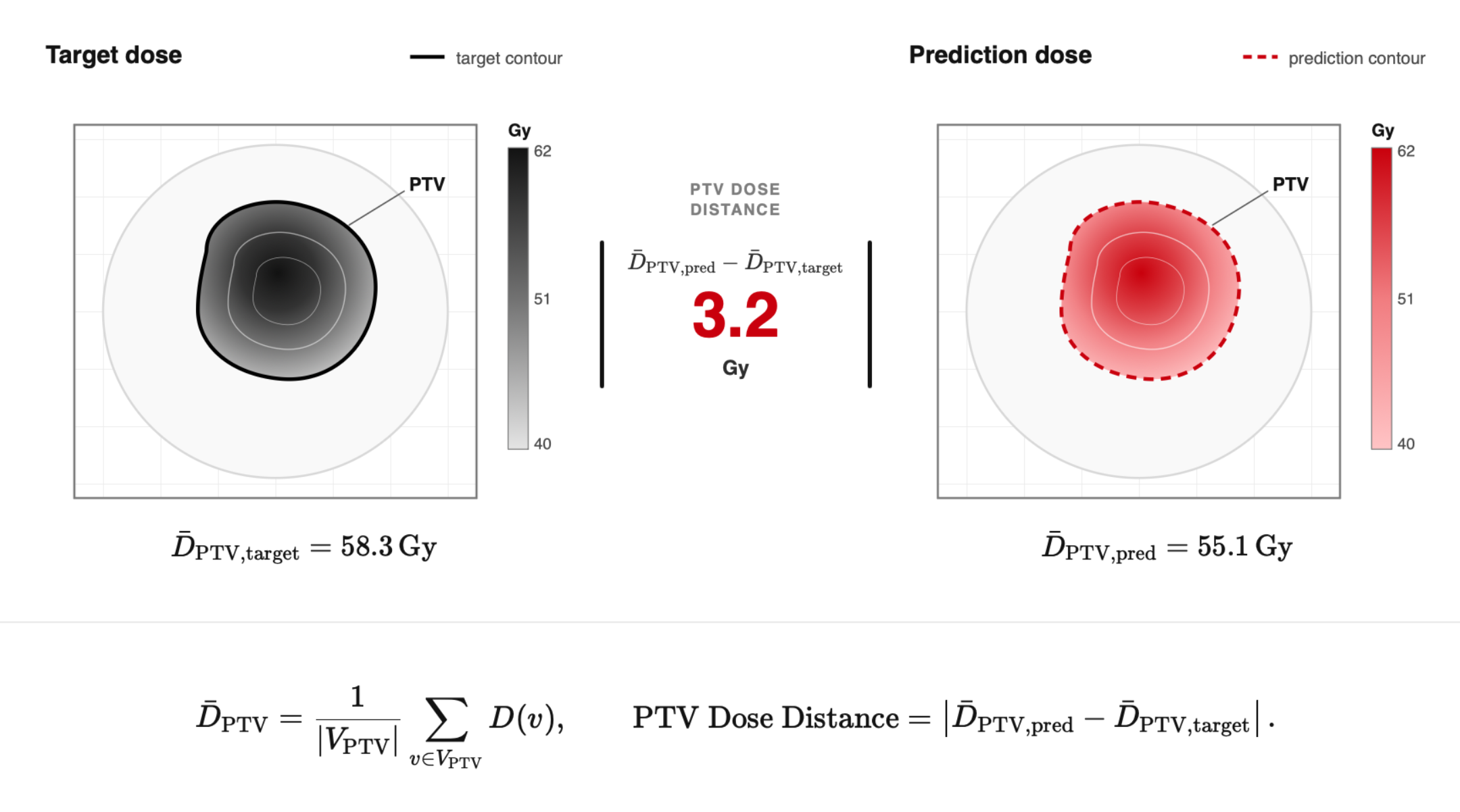PTV mean-dose distance The mean dose is evaluated in the same high-dose PTV for both plans.

For the high-dose PTV volume \(V_{\mathrm{PTV}}\),

\[ \overline{D}_{\mathrm{PTV}} =\frac{1}{\left|V_{\mathrm{PTV}}\right|} \sum_{v\in V_{\mathrm{PTV}}}D(v), \qquad \Delta_{\mathrm{PTV}} =\left|\overline{D}_{\mathrm{PTV,evaluated}} -\overline{D}_{\mathrm{PTV,reference}}\right|. \]

The corresponding reference-free quantity is dvh.compute_mean_dose(dose, ptv).

from dosemetrics.metrics import compare_ptv_dose

distance_gy = compare_ptv_dose(reference, evaluated, ptv_high)

OAR DVH area difference¶

Reference-based · compare_oar_dvh_auc · Gy · lower is better.

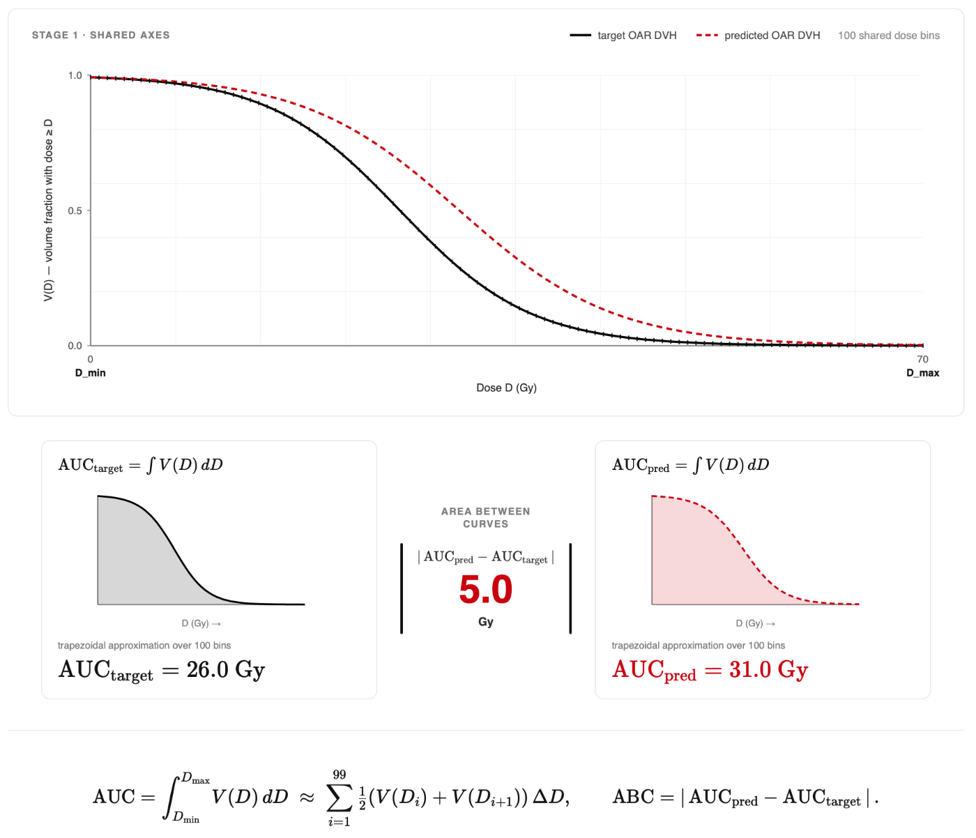OAR DVH AUC distance Both scalar AUCs are evaluated on one common 100-bin dose grid.

\[ \mathrm{ABC} =\left|\mathrm{AUC}_{\mathrm{evaluated}} -\mathrm{AUC}_{\mathrm{reference}}\right|. \]

This is the absolute difference between two scalar areas. It is distinct from the pointwise L1 curve separation implemented by dvh.compare_dvh_area.

from dosemetrics.metrics import compare_mean_oar_dvh_auc, compare_oar_dvh_auc

brainstem_abc_gy = compare_oar_dvh_auc(reference, evaluated, brainstem)
mean_abc_gy = compare_mean_oar_dvh_auc(reference, evaluated, oars)

OpenKBP DVH Score¶

Reference-based · compare_dvh_score · Gy · lower is better.

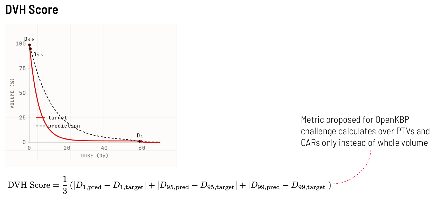OpenKBP DVH Score The score pools target \(D_1\), \(D_{95}\), and \(D_{99}\) with OAR mean-dose and \(D_{0.1\mathrm{cc}}\) criteria.

For all \(M\) criteria,

\[ \mathrm{DVH\ Score} =\frac{1}{M}\sum_{m=1}^{M} \left|m_{\mathrm{evaluated}}-m_{\mathrm{reference}}\right|. \]

from dosemetrics.metrics import compare_dvh_score

score_gy = compare_dvh_score(reference, evaluated, targets=targets, oars=oars)

Other curve comparisons¶

abc_l1 = dvh.compare_dvh_area(reference, evaluated, brainstem, norm="l1")
wasserstein_gy = dvh.compare_dvh_wasserstein(reference, evaluated, brainstem)
ks_statistic, ks_p = dvh.compare_dvh_ks(reference, evaluated, brainstem)
chi2, chi2_p = dvh.compare_dvh_chi_square(reference, evaluated, brainstem)
similarity = dvh.compare_dvh_similarity(
    reference, evaluated, brainstem, method="dice"
)

Multi-plan summaries¶

bins, mean, lower, upper = dvh.compute_dvh_confidence_interval(
    cohort_doses, ptv, confidence=0.95
)
bins, bandwidth = dvh.compute_dvh_bandwidth(cohort_doses, ptv)

See the Metrics API for exact signatures and validation rules.